5. Y2F Interface
YALMIP is a high-level modeling language for optimization in MATLAB. It is very convenient to use for modeling various optimization problems, including convex quadratic programs, for example. YALMIP allows you to write self-documenting code that reads very much like a mathematical description of the optimization model.
To combine the computational efficiency of FORCESPRO with the ease-of-use of
YALMIP, we have created the interface Y2F. Y2F very efficiently detects the
inherent structure in the optimization problem, and uses the FORCESPRO backend
to generate efficient code for it. All you need to do is to replace YALMIP’s
optimizer function, which pre-builds the optimization problem such that
subsequent evaluations become very inexpensive, by Y2F’s optimizerFORCES
function, which is fully API-compatible with optimizer.
This interface is provided with all variants of FORCESPRO, starting with Variant S.
You can read more about the concept of YALMIP’s optimizer here.
Important
The Y2F interface supports convex decision making problems, with or without binary variables.
5.1. Installing Y2F
Y2F is included in the FORCESPRO client. If optimizerFORCES is not found on
your MATLAB path, you need to add the FORCES_PRO/Y2F/Y2F directory to it,
e.g. by typing:
addpath /home/user/FORCES_PRO/Y2F/Y2F
on your MATLAB command prompt.
Of course, you also need a working installation of YALMIP, which you can download from https://yalmip.github.io/download/.
5.2. Generating a solver
A YALMIP model consists of a constraint object, which we name const and an
objective function obj. You can create an optimizer object that has most
of the work YALMIP needs to do before calling a solver (called canonicalization)
already saved. The only parts missing are the parameters of the problem, which
you can specify when calling optimizer:
P = optimizer(Con, Obj, Options, Parameters, WantedVariables); % YALMIP syntax
With Y2F, you can have the same syntax but creating a FORCESPRO solver:
P = optimizerFORCES(Con, Obj, Options, Parameters, WantedVariables, [ParameterNames], [OutputNames]);
where Options is a FORCESPRO codeoptions struct (see the
Solver Options section for more information). The two last arguments
are optional cell arrays of strings specifying the names of the parameters and
the wanted variables. These will be used for naming e.g. the in- and output
ports of the generated Simulink block.
5.3. Calling the solver
There are several ways of calling the generated solver:
1. Using the optimizerFORCES object, which again is API compatible with
YALMIP’s optimizer object:
[wantedVariableValues, exitflag, info = P{Parameters}; % YALMIP syntax
2. Using the generated Matlab (MEX) interface (type help solvername at the
Matlab command prompt for more information):
problem.ParameterName1 = value1; problem.ParameterName2 = value2;
[output, exitflag, info] = solvername(problem);
wantedVariable = output.outputName1;
3. Via the generated Simulink block (see interfaces folder of the generated code).
5.4. Solver info
5.4.1. Exitflags
One should always check whether the solver has exited without an error before
using the solution. Possible values of exitflag are presented in
Table 5.1.
Exitflag |
Description |
|---|---|
|
Optimal solution found to the requested accuracy. |
|
(for branch-and-bound) A feasible point has been identified for which the objective value is no more than (for convex solver) Solver timeout has been reached. |
|
Timeout – maximum number of iterations or maximum computation time of |
|
(only branch-and-bound) Infeasible problem (problems solving the root relaxation to desired accuracy). |
|
(only branch-and-bound) Out of memory – cannot fit branch and bound nodes into pre-allocated memory. |
|
The convex solver could not proceed due to stalled line search. The problem might be infeasible. Otherwise, please submit a bug report to support@embotech.com including all data necessary to reproduce the problem. You can also run |
|
The convex solver could not proceed due to an internal error. The problem might be infeasible. Otherwise, please submit a bug report to support@embotech.com including all data necessary to reproduce the problem. You can also run |
|
License error. If you have generated code with a simulation license, it will run only on the machine from which the code has been generated. In some cases, e.g. when connected to a VPN network, the FORCESPRO license checker produces a false negative. Re-run the code generation script in this case to make sure licensing information is correctly set. |
5.4.2. Additional diagnostics
The solver returns additional information to the optimizer in the info
struct. Some of the fields are described in Table 5.2. Depending
on the method used, there will also be other fields describing the quality of
the returned result.
Info |
Description |
|---|---|
|
Number of iterations. In branch-and-bound mode this is the number of convex problems solved in total. |
|
Total computation time in seconds. |
|
Value of the objective function. |
|
(only branch-and-bound) Number of convex problems solved for finding the optimal solution. Note that often the optimal solution is found early in the search, but in order to certify (sub-)optimality, all branches have to be explored. |
5.5. Performance
A performance measurement for the interface when compared to other solvers called via YALMIP and to the same problem formulated via the low-level interface of FORCESPRO (2 states, 1 input, box constraints, varying horizon) is presented in Figure 5.1. In this example, the code generated directly from YALMIP is about 10 times faster than other solvers, and only a factor 2 slower than the code generated with the low-level interface of FORCESPRO.
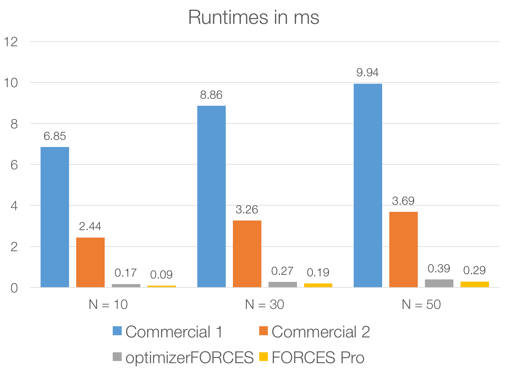
Figure 5.1 Performance comparison of the Y2F interface of FORCESPRO.
5.6. Examples
Y2F interface: Basic example: Learn how to formulate problems in YALMIP easily, and then use the Y2F interface to generate code with FORCESPRO.
Y2F interface: Trajectory Optimization for Quadrotor Flight: A more complex example optimizing the trajectory of a quadrotor within safe flight corridors.